Quick & Dirty Mathematica
Welcome! The point of this tutorial is to teach you how to use Mathematica for menial algebra and calculus.
Fluency in Mathematica has encouraged me to think at a layer of abstraction above algebra, which has increased my enjoyment of courses with a tiresome amount of it. I hope it can do the same for you!
The basics
Mathematica’s most basic functionality is as a calculator. Type 3 + 5, and then press shift-enter to evaluate the expression.
 Mathematica calculates the result, and puts it in
 Out[1]. We can ask Mathematica to multiply the result by 7 by typing %1 * 7.
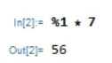
%1 represents the value in Out[1]. You could also have used %, which represents the most recent output.
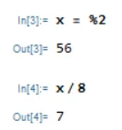
We can assign values to variables in the usual way:
 But the real power of Mathematica is in symbolic calculation.
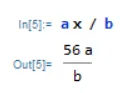 Any string which isn’t already bound to a value is treated as a symbol. By convention, we use lowercase names for variables, because some uppercase letters are reserved (e.g.
 I = Sqrt[-1]).
Be careful: there’s a space in between the a and the x in the input. If you type ax / b, Mathematica will return ax / b, treating ax as the name of a variable. This is a common source of frustration. If Mathematica seems like it’s behaving strangely, make sure you have spaces between your variables!
Once you have a symbolic expression, you can substitute values using rule notation:
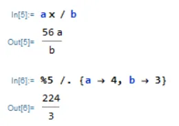 (Mathematica automatically transforms -> into those fancy arrows.)
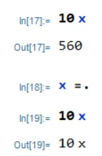
If you’ve previously set a variable that you now want to use as a symbol, you can clear it with =..
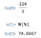
 Functions in Mathematica are called with square brackets. We’ll demonstrate with the
 N function, which converts exact values to decimals.
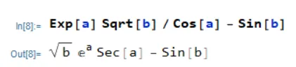
 There are also all the usual math functions,
 as well as differentiation and integration.
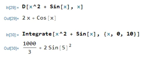 Both
Both D[] and Integrate[] take the variable(s) to integrate or differentiate with respect to as parameters after the expression. If you want a definite integral, you can pass bounds of integration for each variable with {x, 0, 10} instead of x, like we do above.
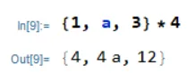
Lists are denoted with curly brackets, and operations are applied elementwise.
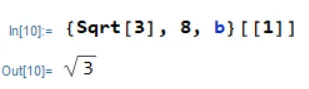
 You can index into lists with double square brackets. Mathematica uses 1-based indexing.
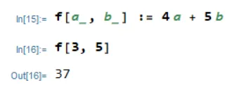
 Mathematica’s functions are defined with the parameters are followed by underscores. Notice that that you assign an implementation to the function with
 :=.
 Ok! Now that we’re done with the basics, we’ll start looking at the stuff that you actually use to solve problems.
The Four Horsemen
When you do homework for classes, you’ll mostly use four functions to wrangle equations: Solve, Reduce, Eliminate, and FullSimplify. I call these the four horsemen of Mathematica.
Solve
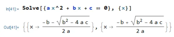
The first horseman is Solve. The most basic functionality of Solve is to take a list of equations and a list of variables, and manipulate the equations to solve for the variables. For example:
 One thing that’s tricky about
 Solve is that all the variables that aren’t solved for must be allowed to range over any value in the solution. For example, Mathematica can’t find a solution here.
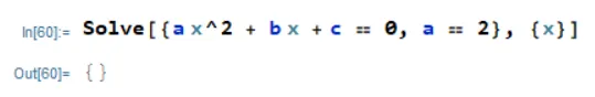 That’s because passing only
 x to Solve tells it to find solutions which admit all values of a, b, c. But there’s no solution that allows all values of a, because a = 2. What we want is for Solve to find values for both x and a that solve the equation for all b, c:

Reduce
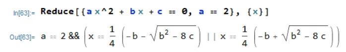
The second horseman is Reduce. Reduce doesn’t require its solution to hold for all values of the unsolved variables. Instead, it will report the conditions that solve the system. With the same input that we gave to the first Solve, Reduce correctly deduces that there is a solution as long as a == 2.
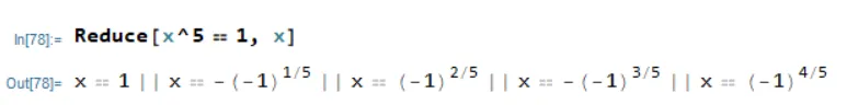
 Reduce can also handle inequalities, domain constraints, and all sorts of other goodies. For example, we can ask for all the fifth roots of unity:
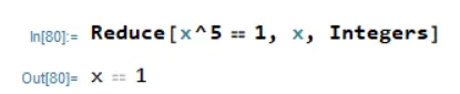
 Or only the integral ones.
Eliminate
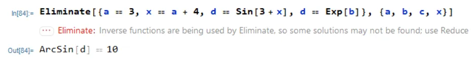
The third horseman is Eliminate. It combines equations to eliminate variables. It’s useful when you have a mess of variables and equations, and you want to reduce your system to a single equation. It takes the list of equations as the first parameter, and the variables to eliminate as the second parameter.
FullSimplify
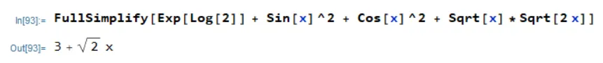
Finally, there’s FullSimplify. It does what you expect, and often transforms complicated results into things that are nicer to write down.
An Example
Now that we’re armed with Solve, Reduce, Eliminate, and FullSimplify, let’s solve a problem.
A rock is throw at an angle theta. It lands 50 meters downrange on a ledge of height h = 20. What was the initial speed of the throw?
We first calculate the integrals of acceleration in the j-hat (vertical) direction:
[a_{\hat{j}} = -g] [v_{\hat{j}} = -gt + v_0 \sin(\theta) ] [s_{\hat{j}} = -\frac{gt^2}{2} + v_0 t \sin(\theta) ]
And then in the i-hat (horizontal) direction:
[a_{\hat{i}} = 0] [v_{\hat{i}} = v_0 \cos(\theta) ] [s_{\hat{i}} = v_0 t \cos(\theta) ]
Now we’re done with the physics—time to plug it into Mathematica.
First we write out the equations as a list. You can get subscripts with ctrl + _ and special characters (like theta) with esc theta esc.
 Then, we eliminate some variables we don’t need.
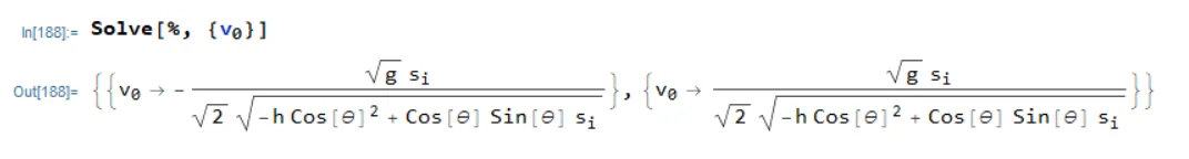
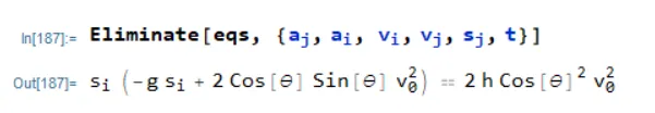 Next, we use
 Solve to rearrange this equation in terms of v0,
 substitute in our values,
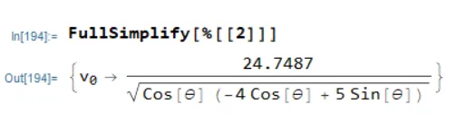
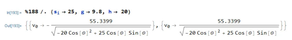 and
and FullSimplify the second result.
 That’s it! Go forth and wrangle some equations!